All about lightning
- Dettagli
- Visite: 24344
|
Scarica (solo in italiano): |
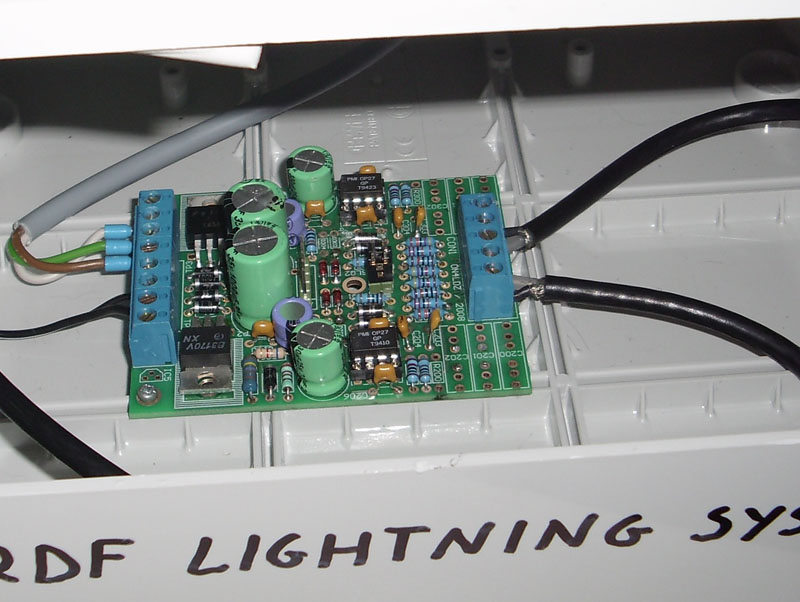
The phenomenon of lightning is actively investigated since 1752, when the American statesman and scientist B.Franklin one of the first established the electrical nature of lightning. As a whole the picture of formation of lightning is as follows. The terrestrial atmosphere is very good dielectric located between two conductors - a surface of the ground from below and the top layers of an atmosphere, including an ionosphere, from above. These layers are passive components of a global electric circuit. Between negatively charged surface of the ground and positively charged top atmosphere the constant potential difference of about 300.000 V is supported. According to the idea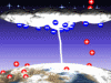 for the first time stated by Wilson in 20th years this ionosphere potential arises from thunder-storms which create global electric "battery". Lightning is a visible electric charge coming from a cloud, going to either another cloud or the earth. Usually, thunder like the sound you are hearing accompanies lightning, especially during a thunderstorm.
Lightning occurs because the bottom of a thundercloud becomes negatively charged, and repels the negative charge of the ground deeper in so the positive charge is more towards the surface. Simple physics says that opposite charges attract, so boom, the lightning takes a one way trip to the closest positively charged item- usually a tree, phone pole, or other high object. Despite of an abundance at present of new devices and methods of research, the microphysical processes leading to charge of storm clouds, remain a subject of disputes.
One of hypothesis, illustrated in animation, connects the lightning appearance with solar activity. The Earth’s upper atmosphere interacts with high energy particles from the sun (called the solar wind) to produce a steady stream of positive ions, which, in turn, rain down onto the Earth’s surface. Nevertheless, the Earth’s total average surface charge does not change. The increase in the Earth’s positive surface charge is cancelled out by the flow of negative electrons from the clouds to the ground during electrical storms. A lightning bolt can deliver a current of 10 million amperes to the Earth’s surface. Electrical storms are connected to solar activity. The sun’s activity peaks every 11 years. When solar wind activity is greater, more positive ions are produced by the solar wind. Thus, more electrical storms are induced on Earth to cancel the increased positive ion flow.
Anatomy of a Lightning Strike
Even in the simple model of a thunderstorm represented in the following picture, lightning strikes are quite complex. 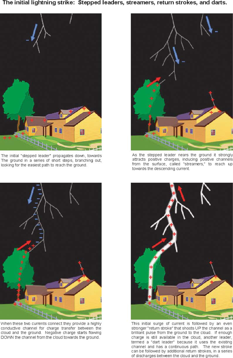
Both negative and positive flashes can occur, but negative flashes are more common. Negative flashes bring negative charge to the ground, while positive flashes bring positive charge to the ground. In negative flashes, the descending current from the cloud moves downward in a series of short jumps, called a “stepped leader.”
The individual steps in this process branch out in different directions, looking for the path of least resistance toward the ground. As a leader gets close to the ground, a corresponding streamer of positive charge moves up from the surface to meet the descending negative current. When these two currents connect they provide a highly conductive channel for charge transfer between the cloud and the ground.
The initial descending negative charge is followed by an even stronger “return stroke” of positive charge from the ground, which seems to move up the channel and into the cloud. The actual charge transfer is, however, done by free electrons so the return stroke is really just a progressive draining of negative charge downward, with the upper limit of the drained path moving upward as electrons flow to the ground. Multiple strokes of dart leaders and return strokes can follow, producing flickering strobe-like flashes of light. The entire multiple discharge sequence of a lightning strike is normally called a flash and is typically made up of two to four separate strokes. In some cases, as many as 15 or more strokes have been observed. The subsequent strokes generally follow the established conducting channel, but the final strike point on the earth’s surface can jump around from strike to strike, with separations of up to several hundred meters or more. These cloud-to-ground flashes are normally called CG lightning, or simply ground lightning.
Electrified thunderstorms are seldom as simple as the idealized dipole. There are complex areas of charge throughout the cloud, resulting in complex electrical fields. There are different types of lightning flashes, including discharges between clouds (intercloud) and within a single cloud (intracloud). Both of these classes of lightning can be grouped together under the single term IC lightning, or cloud lightning. Unlike CG lightning flashes, IC strokes are not followed by return strokes, and they do not carry as much current as is typical for a CG flash. 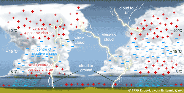
Lightning detection
Cloud discharges and CG flashes both radiate energy over a wide spectrum of frequencies, predominately the radio frequency (RF) bands. During the “stepped” process that creates new channels, there are strong emissions in the very high frequency (VHF) range. High current discharges along previously established channels (“return strokes”) generate powerful emissions in the low frequency (LF) and very low frequency (VLF) ranges. Medium frequency (MF) emissions are centred in the AM radio band and are responsible for the static we hear on 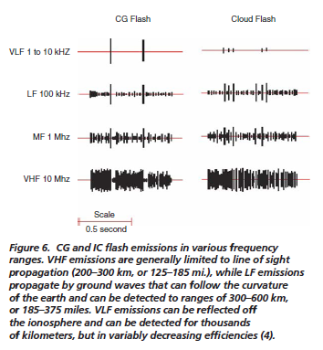 AM radio during lightning storms.
Cloud and ground flashes produce significantly different RF emissions over different time scales, which can be used to distinguish between these two classes of lightning. With their high current and predominately vertically oriented return strokes that generate magnetic fields, CG flashes produce strong signals that can easily be associated with a single position near the point they strike the earth’s surface.
When high currents occur in previously ionized channels during cloud-to-ground flashes, the most powerful emissions occur in the VLF range. VLF (very low frequency) refers to radio frequencies in the range of 3 kHz to 30 kHz. An essential advantage of low frequencies in contrast to higher frequencies is the property that these signals are propagated over thousands of kilometres by reflections from the ionosphere and the ground.
Waves with a frequency between 30 and 3 kHz have a length between 10 and 100 km. An applicable antenna for these frequencies is a small loop antenna of size less than 1/10000 of the wavelength in circumference.
The electric field of the radio waves emitted by cloud-to-ground lightning discharges is mostly oriented vertically, and thus the magnetic field is oriented horizontally. To cover all directions (all-around 360 degree) it is advisable to use more than one loop. A suitable solution can be obtained by two orthogonal crossed loops as they are used for direction finding systems.
The size of the antenna can extremely be reduced by using ferrite rods. But a high number of turns are necessary to reach the same voltage compared with a loop antenna.
This implies that the ferrite antenna has a lower resonance frequency than the loop antenna.
The resonance frequency of the ferrite antenna for wide-band VLF reception should not fall below 100 kHz.
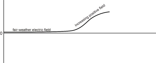
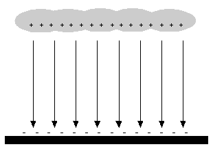
The atmospheric electric field
In the lower atmosphere, the mean atmospheric electric field can be modified due electric charges transport made by convection, corona effect, air humidity and the pollution.
According to Ohm’s Law, under fair weather conditions, is possible to describe the atmospheric electric field in function of the current density:

where E is the local electric field (V/m), s is the electrical conductivity of the air and J is the electrical current density (A/m2).
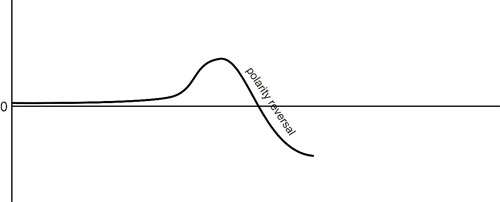
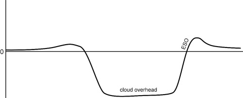
The E.F. in a thunderstorm
The atmospheric electric field for a region where we have a storm is described for the image method, in which it establishes that one charge configuration near a perfect conducting infinite plan can be replaced by the same configuration, its image and a equipotential surface in the place of the conducting plan.
The next equation shows the relation of the lightning distance as function of the local electric field (E), of a charge center (Q) and the charge center height (H):
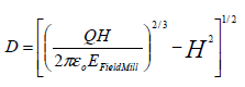
where eo is free space electrical permissivity (8.85x10- 12 C2/N.m2). The thunderstorm charge center height has significant variations. In literature we found that the evaluated height of the charge center in a cloud varies between 3 and 6km, therefore this electric field model assumes a constant height of 6km for the charge center region that originates the electric field that will be measured at the ground by the field mill. Then, the horizontal distance, since the sensor’s site to the charge center evaluated for a typical storm cloud, determines a perimeter in which the occurrence of an atmospheric discharge could be occurred. In this way, the previous equation can evaluate an alert region, based on the value of the electric field measured.
Sensors to detect lightning activities
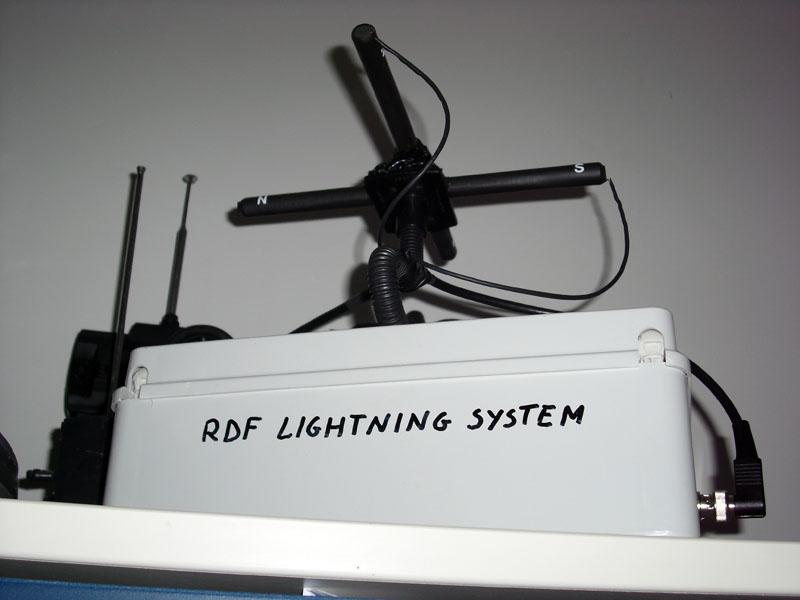
| RDF (Radio Direction finding) Lightning sensor
The DF sensor is an original concept and design by Frank Kooiman and thanks to the help of Daniel Verschueren. The electronics consists of an amplifier which boosts and filters the signal from an antenna and passes it to the soundcard of a computer (Line-in). The direction can be calculated from the two signals measured. It is still not possible to say for certain that the lightning strike occurred at one direction, exactly opposite direction could also have been possible (+180 degrees). This is also due to the fact that we do not know if the lightning strike had a positive or negative charge. If you are working with a single station, a third antenna is therefore necessary to detect the charge and therefore the correct direction of the strike. A single station cannot be used to determine the Now I have in test two ferrite antennas just like the ones used for the TOA system. It's not simple to adapt them to the RDF hardware but some good result is coming :-) You can find information about Lightning Radar on:
|
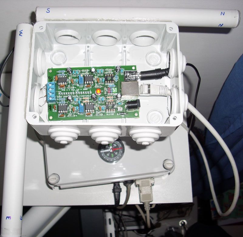
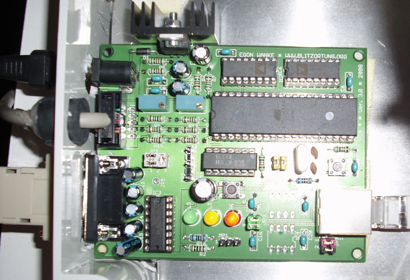
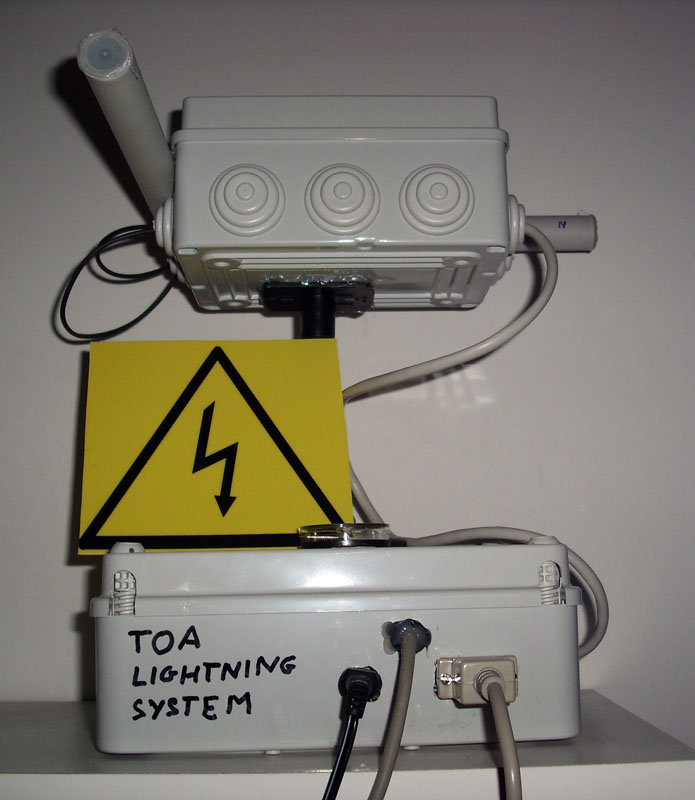
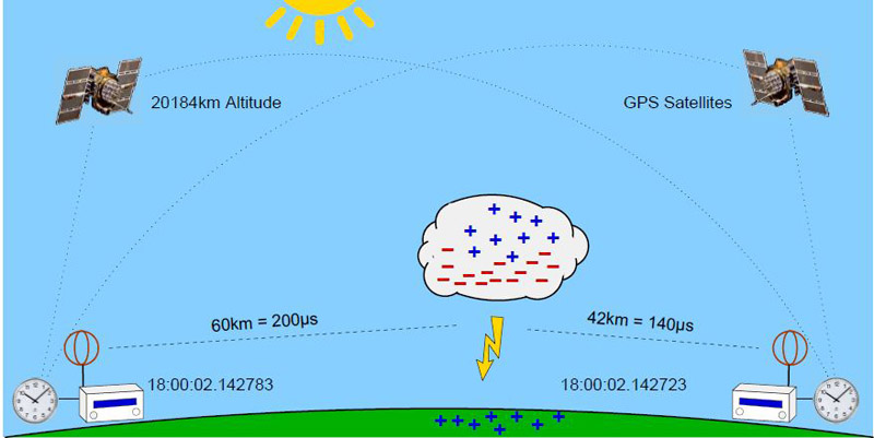
TOA (Time of Arrival) Lightning sensor
The TOA sensor is developed thanks to the Egon Wanke Blitzortung.org project. The TOA (time of arrival) lightning location technique is based on hyperbolic curve calculations.
|

The E-Field Mill
The E-field mill measures the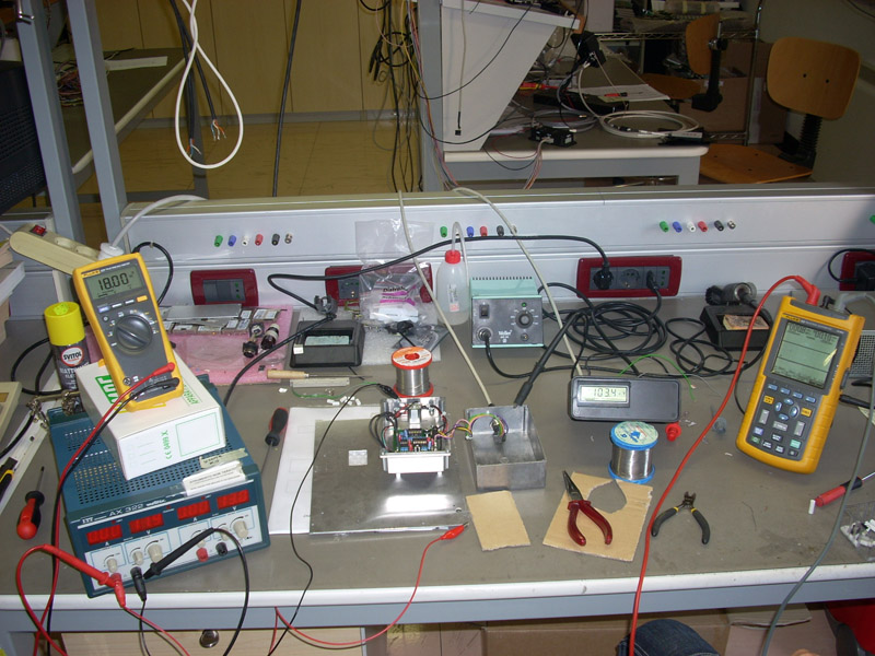 static electric field generated
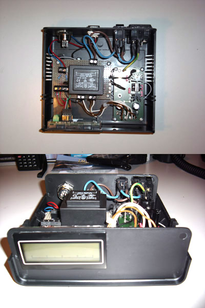 by thunderclouds and can detect the atmospheric conditions which precede lightning.
A field-mill is used to measure an electrical earth field (V/m). A field-mill is based on static electric influence on a conductive plate. If an electrode in an E-field is covered by a rotating wing then the charge is flowing from the electrode to ground. If the electrode is not covered influence charges are flowing back to the electrode.
The current is proportional to E-field.
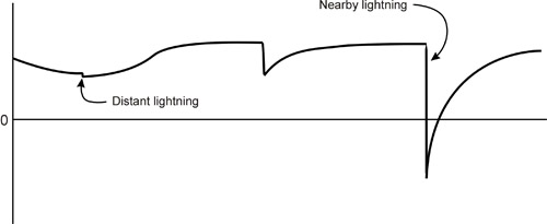
At stable weather E-field is about 100–150 V/m (direction is from atmosphere to earth). Earth is negative and atmosphere is positive. During a lightning there are a lot of charge separations in the cloud. This charging is very strong and under the lightning cloud the E-field can be up to 30000 V/m. Also without lightning strokes the E-field can be very high. This could be used as lightning warning. Depending on cloud type (negative or positive cloud base) E-field is positive or negative. 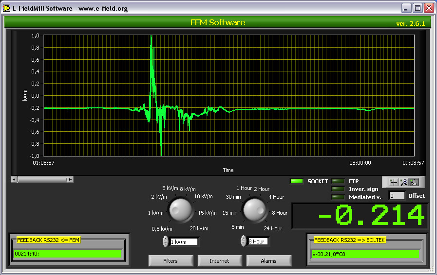
I've developed the software for the E-Field Mill in LabView.
With this one I have the possibilities to send data in graphic images to a specified ftp site, or via socket. It's possible to filter the data received from the field utilizing mediated values, inverting the sign and deciding an Offset.
It's also possible to set two type of alarms, only visible at the moment, for high alarms and very high alarms.
I opened a SourceForge project dedicated to the FEM Software: https://sourceforge.net/projects/femsoftware/
The voltmeter DPM812 used for the original project has become a discontinued product.
|
 ugh you can feel your hair stand on end (if this happens outdoors during a thunderstorm crouch down with your feet together as you are about to be struck by lightning.) An electric field is what attracts your hair to a charged comb or a charged balloon.